Susceptible-Exposed-Infectious-Removed (SEIR) Model Framework with Lesion Expansion

A dynamical systems model for plant disease epidemiology that tracks disease progression through latent, infectious, and removed stages. Supports flexible aging (day or development stage), lesion expansion, and hourly leaf wetness calculations.

Usage

seir(
  wth,
  emergence,
  onset,
  duration,
  H0,
  I0,
  RcA,
  RcT,
  RcOpt,
  p,
  i,
  Sx,
  a = 1,
  rhlim = 90,
  rainlim = 5,
  RRS = NULL,
  RRG = NULL,
  RcW = NULL,
  RRLEX = NULL,
  simple_wetness = TRUE,
  weighted_wetness = FALSE,
  age_driver = c("day", "dvs"),
  thermal_time = NULL,
  infection_window = NULL
)

Arguments

wth

A data.frame of class epicrop.wth from get_wth() or format_wth() containing daily weather data with columns:

Required Columns:

Column	Description
YYYYMMDD	Date (ISO 8601: YYYYMMDD)
DOY	Day of year (1–366)
TEMP	Mean daily temperature (°.RC)
RHUM	Mean daily relative humidity (%)
RAIN	Daily rainfall (mm)

Optional Columns (for advanced features):

Column	Purpose
TMIN	Minimum daily temperature (°.RC); required if simple_wetness = FALSE
TMAX	Maximum daily temperature (°.RC); required if simple_wetness = FALSE
LAT	Latitude; required if simple_wetness = FALSE
LON	Longitude; included in output if present

emergence

Plant emergence (transplanting for rice) date in YYYY-MM-DD format (character).

onset

Days until disease onset after emergence date (1-indexed integer). Value of 1 means disease begins on emergence day. When comparing with legacy SEIR(), use legacy_onset = onset - 1.

duration

Growing season length / simulation duration (integer days). Table 1 in Savary et al. (2012) discusses typical ranges per crop.

H0

Initial healthy sites (integer). Starting condition for compartment H at emergence. Typically 1000 or proportional to plant canopy size.

I0

Initial infective sites (integer). Inoculum at onset day. Becomes infectious after p days.

RcA

Age-based modifier for basic infection rate Rc (numeric matrix). Two-column format:

• Column 1: crop age (days 0 to duration-1 if age_driver="day"; or DVS 0–2 if age_driver="dvs")

• Column 2: modifier (0–1, bounded) Tables 1 and 2 in Savary et al. (2012).

RcT

Temperature modifier for Rc (numeric matrix). Two-column format:

• Column 1: temperature (°.RC)

• Column 2: modifier (0–1, bounded) Tables 1 and 2 in Savary et al. (2012).

RcOpt

Potential infection rate (numeric scalar, unbounded). Rc corrected for removals and optimal conditions. Can be modified to reflect cultivar resistance (see Kim et al. 2015 for details).

p

Latent period duration (days). Can be:

• Integer: constant duration across growing season

• Numeric vector: interpolated against age values

• Function: f(TEMP) to calculate latent days based on daily temperature Table 1 in Savary et al. (2012).

i

Infectious period duration (days). Same flexibility as p. Table 1 in Savary et al. (2012).

Sx

Maximum number of sites per plant/unit canopy (integer). Carrying capacity constraining growth. Table 1 in Savary et al. (2012).

a

Aggregation coefficient (numeric, vector, or function). Controls spatial aggregation of infection:

• a = 1: random infection (binomial); default

• a > 1: aggregated infection (negative binomial) See a - Aggregation Details for full explanation. Can be interpolated against age. Defaults to 1.

rhlim

Relative humidity threshold (%) for leaf wetness (numeric). If RHUM >= rhlim or RAIN >= rainlim, leaves are wet. Savary et al. (2012) used 90. Defaults to 90.

rainlim

Rainfall threshold (mm) for leaf wetness (numeric). If RAIN >= rainlim, leaves are wet regardless of RH. Savary et al. (2012) used 5. Defaults to 5.

RRS

Relative rate of physiological senescence (numeric, vector, or function). Causes healthy sites to senesce independent of disease. Can be:

• Scalar: constant rate (per day)

• Vector or matrix: interpolated against age or DVS

• Function: f(DVS_or_days) for dynamic senescence Table 1 in Savary et al. (2012).

RRG

Relative rate of growth of healthy sites (numeric, vector, or function). Can be:

• Scalar: constant growth rate

• Vector or matrix: interpolated against age or DVS

• Function: f(time) for flexible growth curves Table 1 in Savary et al. (2012).

RcW

Optional modifier curve for leaf wetness effect (numeric matrix). Only used when simple_wetness = FALSE (hourly wetness calculation). Two-column format:

• Column 1: hours of wetness (0–24)

• Column 2: Rc modifier (0–1, bounded) If NULL (default), linear relationship: 0 hrs → modifier 0; 24 hrs → 1. Ignored if simple_wetness = TRUE.

RRLEX

Rate of lesion expansion (numeric, vector, or function). Allows direct H→I conversion bypassing the latent period. Can be:

• Scalar or vector: constant or age-dependent rate

• Function: f(TEMP) or f(DVS) for temperature/age-dependent expansion Set to 0 (default) for standard SEIR (no lesion expansion).

simple_wetness

Logical. Leaf wetness calculation method:

• TRUE (default): Binary (0 or 1) based on rhlim and rainlim thresholds

• FALSE: Hourly calculation (requires TMIN, TMAX, LAT, DOY in wth); applies RcW curve to 0–24 hour range

weighted_wetness

Logical. Only used when simple_wetness = FALSE.

• FALSE (default): Count hours where hourly RH >= rhlim (0–24)

• TRUE: Compute weighted average RH over 24-hour day Defaults to FALSE.

age_driver

Character. Age variable for modifiers:

• "day" (default): 0-indexed days from emergence; RcA and RRS are functions of days

• "dvs": Development stage (0–2); RcA and RRS are functions of DVS; requires thermal_time parameter

thermal_time

List with thermal accumulation parameters (required if age_driver = "dvs"). Must contain:

• base_temp: Base temperature for GDD accumulation (°.RC)

• gdd_to_maturity: Growing degree-days to reach maturity (°.RC·days) Internally computed as: $$DVS = \min\left(2,\ 2 \times \frac{\text{GDD}}{\text{gdd to maturity}}\right)$$

infection_window

Optional list restricting disease onset to a DVS window. Must contain:

• dvs_start: DVS when susceptibility begins (0–2)

• dvs_end: DVS when susceptibility ends (0–2)

• base_temp (optional): Base temperature for GDD (overrides thermal_time if present)

• gdd_to_maturity (optional): GDD to maturity (overrides thermal_time if present) When set, Rc is multiplied by 0 outside the window, preventing infection.

Value

A data.table::data.table() object of class epicrop.sim with one row per day and columns:

State Variables (compartment sizes at end of day):

• simday: Simulation day (1-indexed; 1 = emergence day)

• dates: Calendar date (Date class)

• sites: Healthy sites remaining

• latent: Latent (E) sites

• infectious: Infectious (I) sites

• removed: Removed (R) sites

• senesced: Senesced sites

Flow Variables (daily rate/change):

• rateinf: New infections (H→E) on this day

• rlex: Lesion expansion (H→I directly) on this day

• rtransfer: Transfer from latent to infectious (E→I) on this day

• rremoved: Transfer from infectious to removed (I→R) on this day

• rgrowth: Growth of healthy sites on this day

• rsenesced: Senescence of healthy sites on this day

Derived Variables:

• diseased: Total diseased sites (latent + infectious + removed)

• intensity: Proportion diseased = (latent + infectious) / (sites + latent + infectious); excludes removed and senesced

• lat: Latitude (if provided by wth)

• lon: Longitude (if provided by wth)

Area Under Disease Progress Curve (AUDPC): Accessed via attr(result, "AUDPC"). Computed from intensity using the trapezoidal rule over all days.

Details

This function originated from specific disease models in ‘EPIRICE’ and ‘EPIWHEAT’ to model disease intensity of several rice diseases and two wheat diseases respectively. Given proper values it can be used with other pathosystems as well.

Model Structure

The model tracks five site compartments over time:

• Healthy sites (H): Susceptible to infection

• Latent sites (E): Infected but not yet infectious (duration = p days)

• Infectious sites (I): Can transmit infection (duration = i days)

• Removed sites (R): Diseased but no longer infectious

• Senesced sites (S): Physiologically dead

Daily transitions are driven by:

• Infection rate: \(R_c \times I \times \left(1 - \frac{D}{S_x}\right)^a\) (corrected for crowding & aggregation)

• Latency progression: E→I after p days

• Recovery: I→R after i days

• Growth: H increases based on RRG (if room available)

• Senescence: H and R decrease based on RRS

• Lesion expansion (optional): H→I directly via RRLEX

Mass Balance

At any day, the constraint is: $$ \text{sites}_t + \text{latent}_t + \text{infectious}_t + \text{removed}_t + \text{senesced}_t = H_0 + \text{growth}_t - \text{senescence}_t $$ Accumulated growth is sum(rgrowth) and accumulated senescence is sum(rsenesced). Small numerical deviations may occur due to floating-point arithmetic.

a – Aggregation Details

The infection rate is computed as: $$\text{new infections} = I \times R_c \times \left(1 - \frac{D}{S_x}\right)^a$$ where D = diseased sites, Sx = carrying capacity, and a is the aggregation coefficient:

• a = 1 (random, binomial): Assumes pathogen can access all healthy sites equally. Maximum infection rate per unit of disease.

• a > 1 (aggregated, negative binomial): Pathogen cannot access all healthy sites; infections cluster spatially. Reduces effective infection rate. Refer to Savary et al. (2012) for biological interpretation and fitting guidance.

TMIN/TMAX Details

When simple_wetness = FALSE, the function calculates hourly leaf wetness for 24 hours using TMIN, TMAX, LAT, and DOY in the wth object. The rhlim and rainlim thresholds determine wet hours. A leaf-wetness modifier (RcW) converts wet hours to a 0–1 Rc scale.

When simple_wetness = TRUE, this calculation is skipped; leaf wetness is binary (0 or 1) based solely on daily RHUM and RAIN.

LAT/LON Details

If the wth object contains LAT and LON columns, they are appended to each row of the output for mapping or spatial analysis. Both must be present to be included. By default, get_wth() and format_wth() provide these.

Lesion Expansion Dynamics

When RRLEX > 0, the model adds a direct pathway H→I, bypassing latency: $$\text{rlex}_t = RRLEX \times I_t \times \left(1 - \frac{D}{S_x}\right)$$

Lesion expansion is computed in a two-stage update to avoid circular dependency: (1) compute pre-expansion infectious sites, (2) compute rlex, (3) finalize infectious count. This ensures that Rc-driven infections and lesion expansion are properly sequenced.

References

Sparks, A. H., P. D. Esker, M. Bates, W. Dall' Acqua, Z. Guo, V. Segovia, S.D. Silwal, S. Tolos, and K. A. Garrett, 2008. Ecology and Epidemiology in R: Disease Progress over Time. The Plant Health Instructor. doi:10.1094/PHI-A-2008-0129-02 .

Madden, L. V., G. Hughes, and F. van den Bosch. 2007. The Study of Plant Disease Epidemics. American Phytopathological Society, St. Paul, MN. doi:10.1094/9780890545058 .

Savary, S., Nelson, A., Willocquet, L., Pangga, I., and Aunario, J. 2012. Modeling and mapping potential epidemics of rice diseases globally. Crop Protection, 34: 6–17. doi:10.1016/j.cropro.2011.11.009

Kim, K. H., Cho, J., Lee, Y. H., and Lee, W. S. 2015. Predicting potential epidemics of rice leaf blast and sheath blight in South Korea. Agricultural and Forest Meteorology, 203: 191–207. doi:10.1016/j.agrformet.2015.01.011

Savary, S., Stetkiewicz, S., Brun, F., and Willocquet, L. 2015. Modelling and mapping potential epidemics of wheat diseases. European Journal of Plant Pathology, 142: 771–790. doi:10.1007/s10658-015-0650-7

See also

Disease-specific helper functions:

• bacterial_blight() – Rice bacterial blight

• brown_spot() – Rice brown spot

• leaf_blast() – Rice leaf blast

• sheath_blight() – Rice sheath blight

• tungro() – Rice tungro

• modified_kim_leaf_blast() – Cultivar-adjusted leaf blast

• modified_kim_sheath_blight() – Cultivar-adjusted sheath blight

• leaf_rust() – Wheat leaf rust

• s_tritici_blotch() – Wheat septoria tritici blotch

Utilities:

• get_wth() – Fetch weather data

• format_wth() – Format weather data

Author

Adam H. Sparks, adamhsparks@gmail.com, derived from original code by Robert J. Hijmans, Rene Pangga, Jorrel Aunario, and Kwang-Hyung Kim.

Examples

# Create sample weather data
wth <- get_wth(
  lonlat = c(121.255669, 14.16742),
  dates = "2000-06-30",
  duration = 120L
)

# Run SEIR model with standard parameters (rice leaf blast example)
res <- seir(
  wth = wth,
  emergence = "2000-06-30",
  onset = 20,      # disease begins on day 20
  duration = 120,  # 120-day growing season
  H0 = 1000,       # 1000 initial healthy sites
  I0 = 1,          # 1 initial infected site
  RcA = rbind(c(0, 0.1), c(120, 0.1)),     # age modifier (constant 0.1)
  RcT = rbind(c(25, 1), c(30, 1)),         # temp modifier (optimum at 25\ifelse{latex}{\out{$^\circ$}}{°}.RC)
  RcOpt = 0.5,     # infection rate optimum
  p = 5,           # 5-day latent period
  i = 10,          # 10-day infectious period
  Sx = 10000,      # max 10,000 sites per plant
  a = 1,           # random infection (no aggregation)
  rhlim = 90,      # wetness threshold at 90% RH
  rainlim = 5      # or 5mm rain
)

# Inspect results
head(res)
#>    simday      dates sites latent infectious removed senesced rateinf  rlex
#>     <int>     <IDat> <num>  <num>      <num>   <num>    <num>   <num> <num>
#> 1:      1 2000-06-30  1000      0          0       0        0       0     0
#> 2:      2 2000-07-01  1000      0          0       0        0       0     0
#> 3:      3 2000-07-02  1000      0          0       0        0       0     0
#> 4:      4 2000-07-03  1000      0          0       0        0       0     0
#> 5:      5 2000-07-04  1000      0          0       0        0       0     0
#> 6:      6 2000-07-05  1000      0          0       0        0       0     0
#>    rtransfer rremoved rgrowth rsenesced diseased intensity      lat      lon
#>        <num>    <num>   <num>     <num>    <num>     <num>    <num>    <num>
#> 1:         0        0       0         0        0         0 14.16742 121.2557
#> 2:         0        0       0         0        0         0 14.16742 121.2557
#> 3:         0        0       0         0        0         0 14.16742 121.2557
#> 4:         0        0       0         0        0         0 14.16742 121.2557
#> 5:         0        0       0         0        0         0 14.16742 121.2557
#> 6:         0        0       0         0        0         0 14.16742 121.2557
attr(res, "AUDPC")  # area under disease progress curve
#> [1] 0.02033845

# Example with lesion expansion (H→I bypass)
res_lex <- seir(
  wth = wth,
  emergence = "2000-06-30",
  onset = 20,
  duration = 120,
  H0 = 1000,
  I0 = 1,
  RcA = rbind(c(0, 0.1), c(120, 0.1)),
  RcT = rbind(c(25, 1), c(30, 1)),
  RcOpt = 0.5,
  p = 5,
  i = 10,
  Sx = 10000,
  RRLEX = 0.01     # lesion expansion rate (1% per infectious site per day)
)

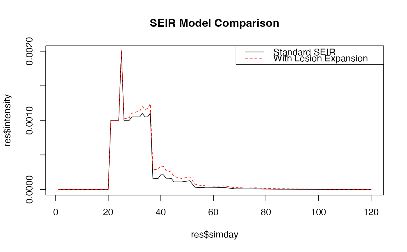
# Compare disease intensity with and without lesion expansion
plot(res$simday, res$intensity, type = "l", main = "SEIR Model Comparison")
lines(res_lex$simday, res_lex$intensity, col = "red", lty = 2)
legend("topright", c("Standard SEIR", "With Lesion Expansion"),
       lty = c(1, 2), col = c("black", "red"))